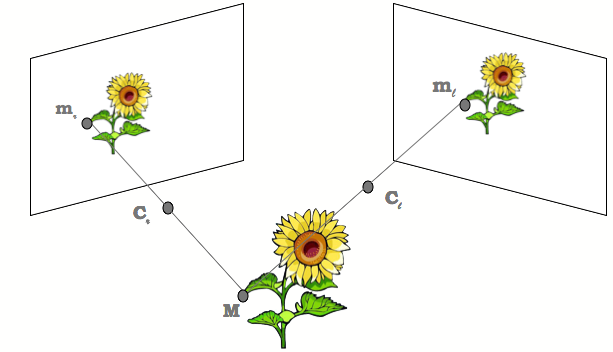
In this project, I extend the feature matching and camera calibration methods to computing camera poses in a two view scenario. This is the first of the series where we deal with computing camera extrinsics from 2 images.
import os
import sys
import cv2
import _pickle as pickle
#import cPickle as pickle
import math
import numpy as np
import matplotlib.pyplot as plt
%matplotlib inline
Lets import all the feature generation and matching from last project
from utils import *The two view images I have used for this project are from here
MIN_MATCH_COUNT = 10

src_image_path = "./imgs/0001.png"
dst_image_path = "./imgs/0002.png"
src_image = cv2.imread(src_image_path, cv2.IMREAD_COLOR)
dst_image = cv2.imread(dst_image_path, cv2.IMREAD_COLOR)

src_gray = cv2.cvtColor(src_image , cv2.COLOR_BGR2GRAY)
dst_gray = cv2.cvtColor(dst_image , cv2.COLOR_BGR2GRAY)

kp1, desc1 = computeDescriptions(src_gray, "feats/{}_feats.kp".format(os.path.basename(src_image_path).split(".")[0]))
kp2, desc2 = computeDescriptions(dst_gray, "feats/{}_feats.kp".format(os.path.basename(dst_image_path).split(".")[0]))

matcher = genMatcher()
knn_matches = matcher.knnMatch(desc1, desc2, 2)
#-- Filter matches using the Lowe's ratio test
ratio_thresh = 0.8
good = []
pts1 = []
pts2 = []
for m,n in knn_matches:
    if m.distance < ratio_thresh * n.distance:
        good.append(m)
        pts2.append(kp2[m.trainIdx].pt)
        pts1.append(kp1[m.queryIdx].pt)

if len(good) <= MIN_MATCH_COUNT:
    print( "Not enough matches are found - {}/{}".format(len(good), MIN_MATCH_COUNT) )
    matchesMask = None
h_,w_, _ = src_image.shapeLets compute the Fundamental matrix using Opencv implementation:
pts1 = np.int32(pts1)
pts2 = np.int32(pts2)

F, mask = cv2.findFundamentalMat(pts1, pts2, cv2.FM_RANSAC )  #FM_LMEDS

# We select only inlier points
pts1 = pts1[mask.ravel()==1]
pts2 = pts2[mask.ravel()==1]Farray([[ 1.15378036e-08, -3.44647723e-07, 5.49071443e-04],
[ 5.56968440e-07, 4.86415551e-08, 4.68608384e-03],
[-7.02721015e-04, -5.34746478e-03, 1.00000000e+00]])
#https://docs.opencv.org/master/da/de9/tutorial_py_epipolar_geometry.html

def drawlines(img1,img2,lines,pts1,pts2):
    ''' img1 - image on which we draw the epilines for the points in img2
        lines - corresponding epilines '''
    r,c = img1.shape
    img1 = cv2.cvtColor(img1,cv2.COLOR_GRAY2BGR)
    img2 = cv2.cvtColor(img2,cv2.COLOR_GRAY2BGR)
    for r,pt1,pt2 in zip(lines,pts1,pts2):
        color = tuple(np.random.randint(0,255,3).tolist())
        x0,y0 = map(int, [0, -r[2]/r[1] ])
        x1,y1 = map(int, [c, -(r[2]+r[0]*c)/r[1] ])
        img1 = cv2.line(img1, (x0,y0), (x1,y1), color,1)
        img1 = cv2.circle(img1,tuple(pt1),5,color,-1)
        img2 = cv2.circle(img2,tuple(pt2),5,color,-1)
    return img1,img2
We then draw the epipolar lines using cv2 eplines
# Find epilines corresponding to points in right image (second image) and
# drawing its lines on left image
lines1 = cv2.computeCorrespondEpilines(pts2.reshape(-1,1,2), 2,F)
lines1 = lines1.reshape(-1,3)
img5,img6 = drawlines(src_gray,dst_gray,lines1,pts1,pts2)

# Find epilines corresponding to points in left image (first image) and
# drawing its lines on right image
lines2 = cv2.computeCorrespondEpilines(pts1.reshape(-1,1,2), 1,F)
lines2 = lines2.reshape(-1,3)
img3,img4 = drawlines(dst_gray, src_gray, lines2,pts2,pts1)

ff, axs = plt.subplots(2,1,figsize=(15,15))
plt.subplot(121),plt.imshow(img5)
plt.subplot(122),plt.imshow(img3)
plt.show()
Ok. Looks like the scheme is working. Here I try writing fundamental_matrix code based on the literature.
def fundamental_matrix_transform(x1, x2):
    n = x1.shape[1]
    if x2.shape[1] != n:
        print("Dimensions mismatch")
        return

    # build matrix for equations
    A = np.zeros((n,9))
    for i in range(n):
        A[i] = [x1[0,i]*x2[0,i], x1[0,i]*x2[1,i], x1[0,i]*x2[2,i],
                x1[1,i]*x2[0,i], x1[1,i]*x2[1,i], x1[1,i]*x2[2,i],
                x1[2,i]*x2[0,i], x1[2,i]*x2[1,i], x1[2,i]*x2[2,i] ]

    # compute linear least square solution
    U,S,V = np.linalg.svd(A)
    F = V[-1].reshape(3,3)

    # constrain F
    # make rank 2 by zeroing out last singular value
    U,S,V = np.linalg.svd(F)
    S[2] = 0
    F = np.dot(U,np.dot(np.diag(S),V))
    return F/F[2,2]
F2 = compute_fundamental().estimate(pts1, pts2 )
F2array([[-0.37796417, -0.01470622, -0.06126958],
[-0.14719857, -0.00165243, -0.09648122],
[-0.14306451, -0.06298112, 1. ]])
Lets confirm our F matrix is valid
# Find epilines corresponding to points in right image (second image) and
# drawing its lines on left image
lines1 = cv2.computeCorrespondEpilines(pts2.reshape(-1,1,2), 2,F2)
lines1 = lines1.reshape(-1,3)
img5,img6 = drawlines(src_gray,dst_gray,lines1,pts1,pts2)

# Find epilines corresponding to points in left image (first image) and
# drawing its lines on right image
lines2 = cv2.computeCorrespondEpilines(pts1.reshape(-1,1,2), 1,F2)
lines2 = lines2.reshape(-1,3)
img3,img4 = drawlines(dst_gray, src_gray, lines2,pts2,pts1)

ff, axs = plt.subplots(2,1,figsize=(15,15))
plt.subplot(121),plt.imshow(img5)
plt.subplot(122),plt.imshow(img3)
plt.show()
Not bad. We also try to utilize SkLearns measure method to test for eplipolar consistency
from skimage.transform import FundamentalMatrixTransform
from skimage.measure import ransacmodel, inliers = ransac((pts1,pts2),
FundamentalMatrixTransform, min_samples=8,
residual_threshold=1, max_trials=5000)F3 = model.paramsmodel.paramsarray([[-3.31331166e-09, 1.23636098e-07, -1.76227099e-04],
[-1.72603899e-07, -1.33622884e-08, -9.08808472e-04],
[ 2.12593170e-04, 1.05536962e-03, -2.12112527e-01]])
# Find epilines corresponding to points in right image (second image) and
# drawing its lines on left image
lines1 = cv2.computeCorrespondEpilines(pts2.reshape(-1,1,2), 2,F3)
lines1 = lines1.reshape(-1,3)
img5,img6 = drawlines(src_gray,dst_gray,lines1,pts1,pts2)

# Find epilines corresponding to points in left image (first image) and
# drawing its lines on right image
lines2 = cv2.computeCorrespondEpilines(pts1.reshape(-1,1,2), 1,F3)
lines2 = lines2.reshape(-1,3)
img3,img4 = drawlines(dst_gray, src_gray, lines2,pts2,pts1)

ff, axs = plt.subplots(2,1,figsize=(15,15))
plt.subplot(121),plt.imshow(img5)
plt.subplot(122),plt.imshow(img3)
plt.show()
Ok lets get to the crux of the matter. We load the camera instrinsics. These 2 images are distortions corrected so we dont have to worry about them
K = np.loadtxt("./calib.txt")Here is the quick code to decompose Essential matrix based on HZ (9.12)
def unitDeterminantCheck(M):
    return abs(np.linalg.det(M)) - 1.0 < 1e-7

def decompEssentialMatrix(E):
    # svd::modify_A
    _, u, vt = cv2.SVDecomp(E, 1)
    if np.linalg.det(vt) < 0:
        vt *= -1
    if np.linalg.det(u) < 0:
        u *= -1
    """R = svd.u * Mat(W) * svd.vt;"""
    W = np.array([[0,-1,0],[1,0,0],[0,0,1]]);
    R1 = np.matmul( u, np.matmul( W, vt ) )
    R2 = np.matmul( u, np.matmul( W.T, vt ) )
    t = u[:,-1]
    if not unitDeterminantCheck(R1) and not unitDeterminantCheck(R2):
        print("Not rotation matrices")
    return R1, R2, t
Lets assume P0 as initlal pose. Then,
Kinv = np.linalg.inv(K)
"""Pose for 1st view"""
P0 = np.eye(3,4)

""""E = K.T * F * K"""
E = np.matmul( K.T , np.matmul( F, K ) )
R1, R2, t = decompEssentialMatrix(E)


"""Poses for 2nd view. One possilbe solutions based on chirality"""

P1 = np.column_stack( [ R1, t ] )P1array([[ 0.90696359, -0.06571734, -0.41605082, 0.9862451 ],
[-0.05300211, -0.99770858, 0.042052 , -0.03347639],
[-0.41786102, -0.01608806, -0.90836851, -0.16186392]])
References
Multiple View Geometry in Computer Vision (second edition), R.I. Hartley and A. Zisserman, Cambridge University Press, ISBN 0-521-54051-8